Archaeological sites on the seabed, sunken ships, plant and coral growth, and the biomass or size of fish populations are among the other points of interest for underwater 3D observations. To achieve 3D reconstruction underwater, various contactless approaches have been used. Sonar systems, laser scanning, time-of-flight (ToF) cameras, and photogrammetry are some examples.
While sonar devices can quickly survey huge regions over great distances, they have lower measurement precision than optical sensors.
In various research efforts, structured illumination has made precise underwater measurements, working well at close ranges and with small items.
These systems have shown promise for the reconstruction technique’s high measurement accuracy. However, the pattern projectors in these systems often have insufficient light power to meet the demands of difficult industrial inspection activities.
They must, for example, have a wide field of vision, be capable of measuring across long distances, be able to handle the limited time available for scanning and data processing, and, ultimately, be able to build real-time 3D surface models of the observed item.
This necessitates a high lighting power for structured light patterns, a cooling concept for the dissipation of created heat, and high-power computer equipment for processing the vast amount of data,regarding accurate camera technology.
Utilizing video streams from an action sport cam and structure from motion (SfM) technology, low-budget 3D reconstruction and merging were successfully applied to underwater 3D seabed surveys in nearshore shallow waters.
These innovative approaches for creating 3D models with a moving camera or a scanner were presented and published in the MDPI journal applied sciences.
The goal was to see how a new stereo scanning technique with structured illumination could be used for precise, constant 3D capturing and modeling of underwater structures throughout medium-range measurement distances (up to 3 meters) and fields of view of roughly 1 m2.
Methodology
According to the needs of potential users, researchers designed a sensor system based on defined light illumination for an underwater 3D inspection system for industrial structures. Examination of oil and gas pipelines, offshore windmill foundations, anchor chains, and other technological constructions is one of its primary applications. It can be installed on a remotely operated vehicle (ROV) and from a ship.
The technology was designed to be used in a laboratory setting (Figure 1).
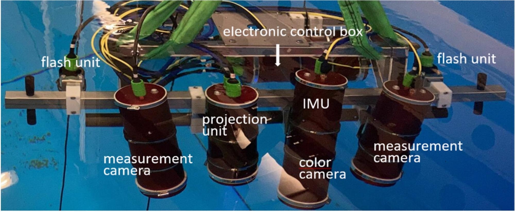
Figure 1. Laboratory setup of UWS. Image Credit: Bräuer-Burchardt, et al., 2022
A PC workstation for management and collection of measurement data, as well as a power supply, is another essential piece of equipment that can be mounted on the vessel and attached to the UWS. The cameras and lenses are readily available on the market. The projection unit was developed by Fraunhofer IOF and consists primarily of an LED light source, a revolving slide (GOBO wheel) and motor, a projection lens, and control electronics.
The aperiodic fringe projection GOBO unit generates measurement data from the stereo camera picture stream. Employing standardized camera geometries, the basic principle of triangulation of comparable points in camera images is used.
A detailed theoretical geometrical analysis of the optical sensor components (cameras, lenses, and glass cover), as well as the extra key conditions and features, was undertaken to get ideal geometric 3D sensor modeling.
A series of ArUco and circle markers in a plane-near configuration were used to calibrate the sensor in a water basin (Figure 2).
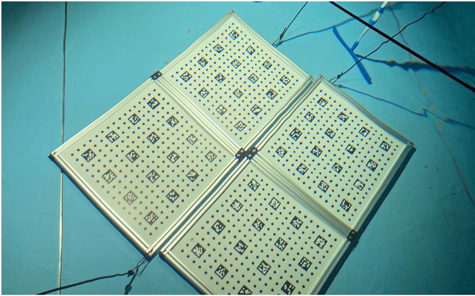
Figure 2. Sheets with ArUco markers combined with circle grids are used for calibration. Image Credit: Bräuer-Burchardt, et al., 2022
Static measurements of supplied specimens, including a ball bar and a plane-normal with calibrated measures, were used to assess calibration. After analyzing the ball bar’s evaluation readings, a 3D error-compensation function was created and employed as the calibration’s final step.
The pixels representing a particular object point shift due to the relative movement between the recording camera and the visible measurement item. When this shift surpasses one or two pixels per sequence recording, the image points get smeared, similar to when an average filter operator is used. As a result, 3D measurement mistakes occur.
A registration technique with multiple stages is utilized for further refining of the motion trajectory, based on the preliminary calculation of the motion trajectory via visual-inertial odometry.
The 3D data is filtered in advance of registration to lower the size of the 3D point cloud and produce an equalized spatial distribution of the selected points.
With local optimization of the trajectory and enhancement of the final 3D map, each 3D point cloud is progressively recorded against its predecessors using an iterative closest point algorithm (ICP).
Results and Discussion
Figure 3 depicts the specimen and sensor device in a basin throughout specimen assessment measurement.
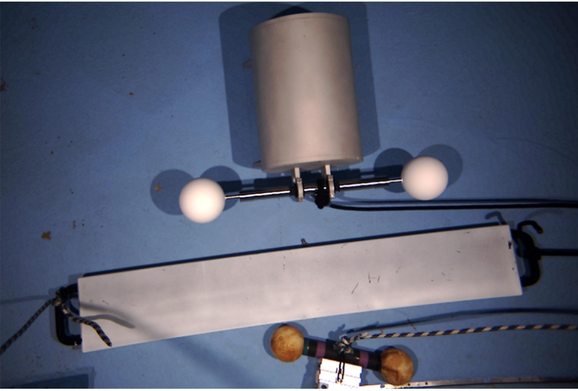
Figure 3. Specimen ball bars, plane-normal, and cylinder during evaluation measurements. Image Credit: Bräuer-Burchardt, et al., 2022
The first findings of the ball-bar length measurement revealed a large proportional relationship between measurement distance and length measurement inaccuracy.
Table 1 shows the findings of the ball bar’s static measurements taken during underwater testing. A 3D correction function is used for the entire set of 3D measurement points during refinement.
Table 1. Results of spherical diameter and ball-bar measurements without and with error compensation (refinement). Standard deviation values of the single measurements are obtained from two to four independent measurements. Source: Bräuer-Burchardt, et al., 2022
| Distance [m] |
R1 [mm] 1 |
R1 Refined [mm] 1 |
R2 [mm] 1 |
R2 Refined [mm] 1 |
Length [mm] 1 |
Length Refined [mm] 1 |
| 1.5 |
50.303 ± 0.01 |
50.412 ± 0.07 |
50.174 ± 0.05 |
50.233 ± 0.01 |
497.355 ± 0.06 |
497.702 ± 0.07 |
| 1.6 |
50.360 ± 0.01 |
50.390 ± 0.02 |
50.191 ± 0.03 |
50.239 ± 0.01 |
497.353 ± 0.01 |
497.624 ± 0.01 |
| 1.7 |
50.372 ± 0.01 |
50.444 ± 0.02 |
50.147 ± 0.03 |
50.201 ± 0.04 |
497.457 ± 0.01 |
497.652 ± 0.01 |
| 1.8 |
50.368 ± 0.05 |
50.380 ± 0.01 |
50.193 ± 0.01 |
50.211 ± 0.03 |
497.467 ± 0.01 |
497.574 ± 0.01 |
| 1.9 |
50.361 ± 0.03 |
50.401 ± 0.08 |
50.225 ± 0.01 |
50.234 ± 0.03 |
497.533 ± 0.03 |
497.572 ± 0.04 |
| 2.0 |
50.448 ± 0.01 |
50.445 ± 0.01 |
50.245 ± 0.01 |
50.252 ± 0.02 |
497.614 ± 0.06 |
497.577 ± 0.07 |
| 2.1 |
50.559 ± 0.01 |
50.530 ± 0.01 |
50.225 ± 0.02 |
50.245 ± 0.06 |
497.689 ± 0.05 |
497.578 ± 0.04 |
| 2.2 |
50.515 ± 0.02 |
50.427 ± 0.05 |
50.352 ± 0.01 |
50.286 ± 0.01 |
497.775 ± 0.02 |
497.593 ± 0.04 |
| 2.3 |
50.530 ± 0.03 |
50.504 ± 0.07 |
50.353 ± 0.04 |
50.276 ± 0.05 |
497.874 ± 0.02 |
497.591 ± 0.01 |
| 2.4 |
50.611 ± 0.14 |
50.577 ± 0.04 |
50.425 ± 0.02 |
50.314 ± 0.04 |
498.002 ± 0.02 |
497.648 ± 0.02 |
| average |
50.443 ± 0.11 |
50.451 ± 0.07 |
50.253 ± 0.09 |
50.249 ± 0.04 |
497.612 ± 0.22 |
497.611 ± 0.05 |
1 Reference (calibrated) values for R1 and R2 are 50.202 mm and 50.193 mm, respectively. True length of ball bar is 497.612 mm.
Figure 4 depicts the ball-bar length measurement findings as a function of measurement distance. The length values are visibly drifting; however, refining substantially lowers this effect. Figure 5 depicts three examples of plane-normal measurements (1.7 meters, 2.0 meters, and 2.4 meters).
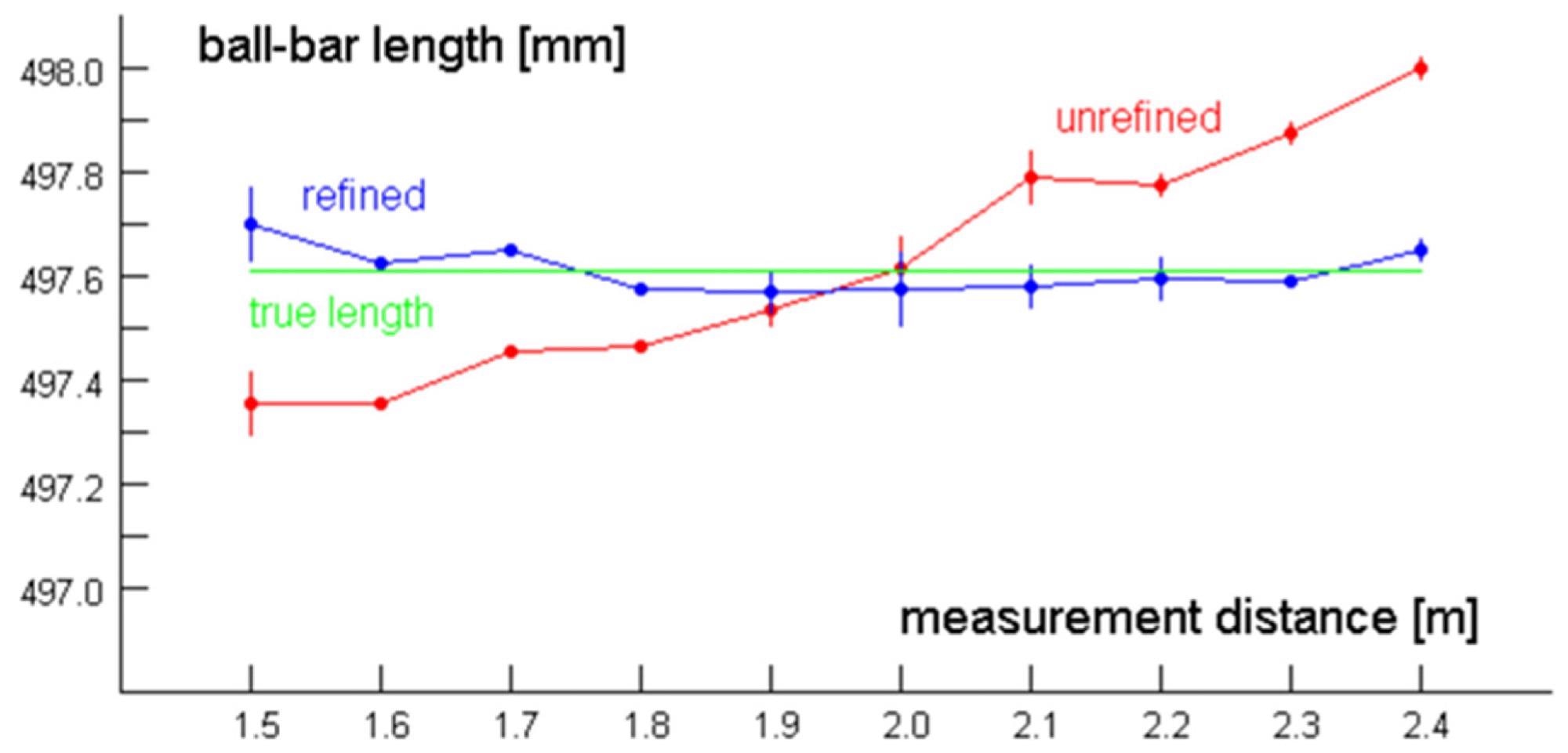
Figure 4. Ball-bar length measurement results depending on object distance. Image Credit: Bräuer-Burchardt, et al., 2022
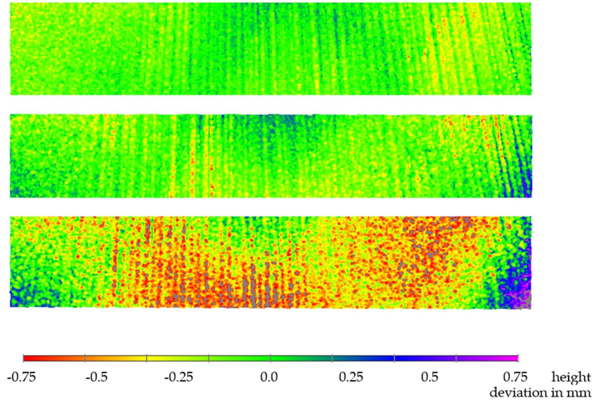
Figure 5. False-color representation of flatness deviation: measurement distance of 1.7 m (above), 2.0 m (middle), and 2.4 m (below). Image Credit: Bräuer-Burchardt, et al., 2022
Table 2 illustrates the distortion of the 3D measurement points on the surfaces of sphere1 and sphere2, as well as the plane’s normal surface, as a function of object distance. Noise increases as the measuring distance increases, as anticipated.
Table 2. Results of noise determination on sphere surfaces and plane normal depending on object distance; refinement does not have any influence on the noise values. Source: Bräuer-Burchardt, et al., 2022
| Distance [m] |
Noise on Sphere1 [mm] |
Noise on Sphere2 [mm] |
Noise on Plane [mm] |
| 1.5 |
0.074 ± 0.01 1 |
0.074 ± 0.01 1 |
0.065 ± 0.02 2 |
| 1.6 |
0.059 ± 0.01 |
0.073 ± 0.02 |
0.075 ± 0.02 |
| 1.7 |
0.062 ± 0.01 |
0.075 ± 0.01 |
0.070 ± 0.01 |
| 1.8 |
0.085 ± 0.01 |
0.081 ± 0.01 |
0.080 ± 0.02 |
| 1.9 |
0.071 ± 0.01 |
0.096 ± 0.01 |
0.090 ± 0.01 |
| 2.0 |
0.078 ± 0.01 |
0.078 ± 0.01 |
0.085 ± 0.01 |
| 2.1 |
0.087 ± 0.01 |
0.089 ± 0.01 |
0.095 ± 0.01 |
| 2.2 |
0.114 ± 0.01 |
0.093 ± 0.01 |
0.115 ± 0.03 |
| 2.3 |
0.098 ± 0.01 |
0.089 ± 0.01 |
0.120 ± 0.02 |
| 2.4 |
0.133 ± 0.01 |
0.104 ± 0.01 |
0.130 ± 0.02 |
| average |
0.086 ± 0.23 |
0.085 ± 0.13 |
0.080 ± 0.13 |
1 Standard deviation values on spheres are obtained from two to four independent measurements.
2 Standard deviation values on planes are obtained from ten independent surface positions.
At a velocity of 0.2 m/s and a 375 Hz 2D framerate, Figure 6 displays the 3D point clouds of the measuring object cylinder, two ball bars, and a plaster bust with and without motion compensation. The findings at 1.0 m/s were not entirely satisfactory, and they should be developed in the future.
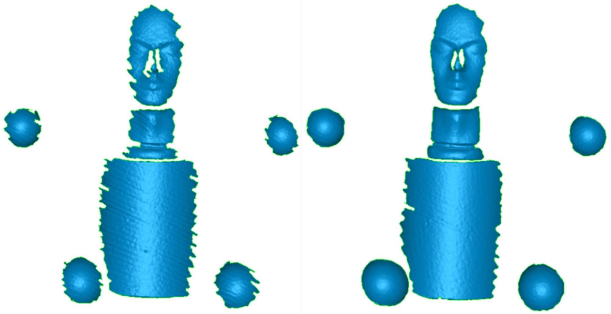
Figure 6. 3D measurement results of the reconstruction of the air measurement with sensor velocity of 0.2 m/s without motion compensation (left) and with motion compensation (right). Note the higher completeness at the margins of the objects with motion compensation. Image Credit: Bräuer-Burchardt, et al., 2022
In the case of a plastic pipe, Figure 7 summarizes the output of manual and automatic motion compensation at 0.7 m/s velocities contrasted to the measured data without motion compensation (left).
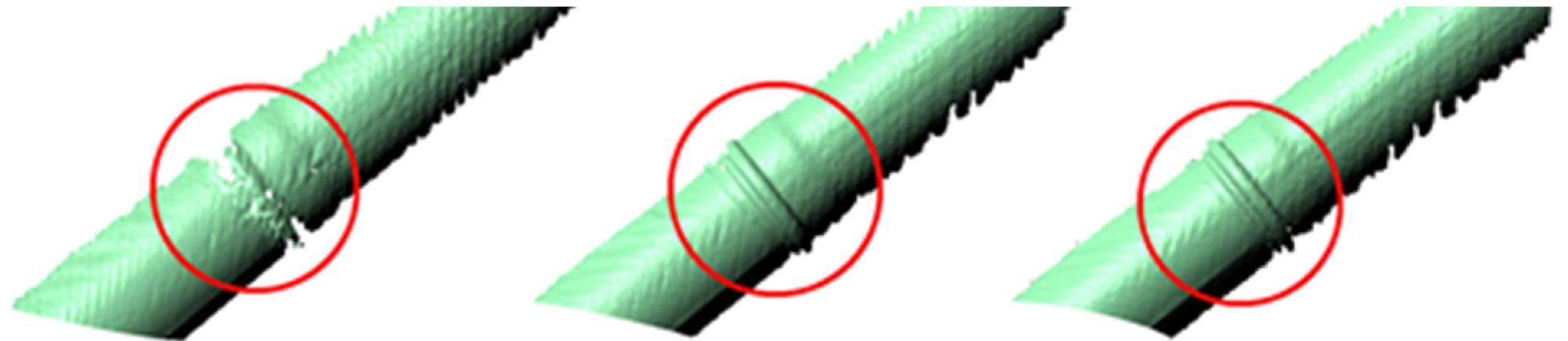
Figure 7. 3D reconstruction result of underwater pipe measurement at 0.7 m/s sensor velocity without motion compensation (MC) (left), manual MC (middle), and automatic MC (right). Image Credit: Bräuer-Burchardt, et al., 2022
The standard deviations of the 3D points from the fitted sphere and cylinder shapes are presented in Table 3. The standard deviation is significantly reduced when motion correction is used. Automatic motion compensation produces outcomes that are equivalent to manual motion compensation.
Table 3. Results of standard deviations of the 3D points from the fitted sphere and cylinder shape depending on sensor velocity and compensation method. Source: Bräuer-Burchardt, et al., 2022
| Velocity |
Compensation Method |
Standarddev. Sphere-Fit |
Point Number on Sphere |
Standarddev. Cylinder-Fit |
Point Number on Cylinder |
| 0.1 m/s |
No |
0.39 mm |
6800 |
0.31 mm |
69,000 |
| 0.1 m/s |
Manually |
0.31 mm |
7100 |
0.32 mm |
69,000 |
| 0.1 m/s |
Automatically |
0.33 mm |
7100 |
0.32 mm |
69,000 |
| 0.7 m/s |
No |
0.52 mm |
3200 |
0.39 mm |
47,500 |
| 0.7 m/s |
Manually |
0.36 mm |
5200 |
0.34 mm |
49,600 |
| 0.7 m/s |
Automatically |
0.32 mm |
6000 |
0.34 mm |
49,600 |
A triaxial gantry system was used to conduct additional dynamic recordings. A pipeline, as well as the ball-bar specimen and plane normal, was lowered into the sea. The underwater setting is shown in Figure 8’s left image.
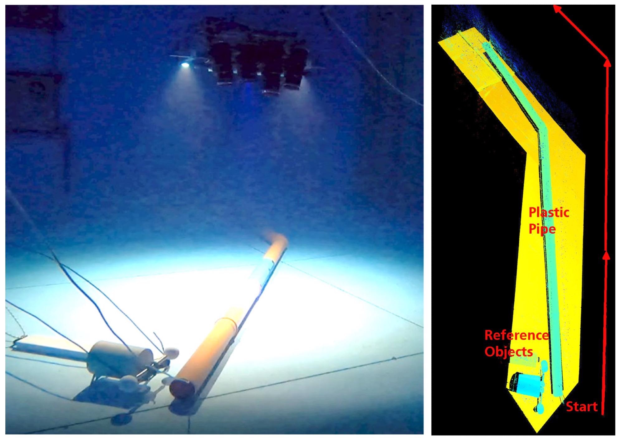
Figure 8. Photograph of the sensor, pipe, and specimen (left) and false-color representation of the modeling result after merging of the continuously recorded 3D data sets (right). Image Credit: Bräuer-Burchardt, et al., 2022
Conclusion
Researchers introduced a novel underwater 3D scanning system suited for offshore inspection applications (up to 1000 m depth). The sensor continually records the surface an item and creates a 3D model of the scanned object in real time by traveling over it at speeds of up to 0.7 m/s. In a water basin, the sensor was assessed under clear water acquisition parameters.
The findings of the current structured-light-based underwater 3D sensor described here signal a turning point in developing such sensor systems in terms of measurement accuracy. The systematic measurement error would be in the same range of accuracy as 3D air scanners of comparable measuring volume, according to the conclusions of static measurements of the specimens.
The novel system has a significantly larger measuring volume, long object distance, and shorter exposure time than earlier setups or devices based on the same 3D data gathering principles (Table 4)
Table 4. Parameters of the 3D scanner compared previous devices based on structured illumination. Source: Bräuer-Burchardt, et al., 2022
| Device |
Measurement Volume |
Measurement Distance |
Exposure Time |
| Ref [32] |
0.5 m × 0.4 m × 0.4 m 1 |
1.0 ± 0.20 m |
not specified |
| Ref [33] |
0.5 m × 0.4 m × 0.2 m 1 |
1.0 ± 0.10 m |
0.8 … 10 s |
| Ref [34] |
0.25 m × 0.2 m × 0.1 m |
0.4 ± 0.05 m |
15 ms |
| UWS |
0.9 m × 0.8 m × 0.8 m |
2.0 ± 0.40 m |
1 … 2.6 ms |
1 estimation according to the provided data in the cited paper.
The random errors found are within the predicted range.
Expanding the experiments to offshore measurements under typical application settings is the key objective for future development. Water turbidity, temperature, and salinity should all be considered in these tests.
The effects of particles in water on scattering should also be investigated. Researchers propose to evaluate the UWS sensor system in an adequate compression chamber to simulate use at a 1000 m depth before conducting real offshore trials.
Another objective for future work is to develop a suitable calibration procedure that can be carried out effectively offshore, even in bad weather.
Journal Reference:
Bräuer-Burchardt, C., Munkelt, C., Bleier, M., Heinze, M., Gebhart, I., Kühmstedt, P., Notni, G. (2022) A New Sensor System for Accurate 3D Surface Measurements and Modeling of Underwater Objects. Applied Sciences, 12(9), p. 4139. Available Online: https://www.mdpi.com/2076-3417/12/9/4139/htm.
References and Further Reading
- Tetlow, S & Allwood, R L (1994) Use of a laser stripe illuminator for enhanced underwater viewing. In: Ocean Optics XII 1994, Bergen, Norway, 26 October; 2258. doi.org/10.1117/12.190098.
- McLeod, D., et al. (2013) Autonomous inspection using an underwater 3D LiDAR. In: 2013 OCEANS, San Diego, CA, USA, 23–27 September; IEEE: New York, NY, USA
- Canciani, M., et al. (2003) Low cost digital photogrammetry for underwater archaeological site survey and artifact insertion. The case study of the Dolia wreck in secche della Meloria-Livorno-Italia. The International Archives of the Photogrammetry, Remote Sensing and Spatial Information Sciences, 34, pp. 95–100. Available at: https://halshs.archives-ouvertes.fr/halshs-00271413
- Roman, C., et al. (2010) Application of structured light imaging for high resolution mapping of underwater archaeological sites. In Oceans’10 IEEE Sydney, Sydney, NSW, Australia, 24–27; doi.org/10.1109/OCEANSSYD.2010.5603672.
- Drap, P (2012) Underwater photogrammetry for archaeology. In: Special Applications of Photogrammetry; Da Silva, D.C., Ed.; InTech: London, UK.. doi.org/10.5772/33999.
- Eric, M., et al. (2013) The impact of the latest 3D technologies on the documentation of underwater heritage sites. In: 2013 Digital Heritage International Congress (DigitalHeritage), Marseille, France, 28 October–1 November;2. doi.org/10.1109/DigitalHeritage.2013.6744765.
- Menna, F., et al. (2018) State of the art and applications in archaeological underwater 3D recording and mapping. Journal of Cultural Heritage, 33, pp. 231–248. doi.org/10.1016/j.culher.2018.02.017.
- Korduan, P., et al. (2003) Unterwasser-Photogrammetrie zur 3D-Rekonstruktion des Schiffswracks “Darßer Kogge”. Photogrammetrie, Fernerkundung, Geoinformation, 5, pp. 373–381.
- Bythell, J. C., et al. (2001) Three-dimensional morphometric measurements of reef corals using underwater photogrammetry techniques. Coral Reefs, 20, pp. 193–199. doi.org/10.1007/s003380100157.
- Harvey, E., et al. (2003) The accuracy and precision of underwater measurements of length and maximum body depth of southern bluefin tuna (Thunnus maccoyii) with a stereo–video camera system. Fisheries Research, 63(3), pp. 315–326. doi.org/10.1016/S0165-7836(03)00080-8.
- Dunbrack, R L (2006) In situ measurement of fish body length using perspective-based remote stereo-video. Fisheries Research, 82(1–3), pp. 327–331. doi.org/10.1016/j.fishres.2006.08.017.
- Costa, C., et al. (2006) Extracting fish size using dual underwater cameras. Aquacultural Engineering, 35(3), pp. 218–227. doi.org/10.1016/j.aquaeng.2006.02.003.
- Galceran, E., et al. (2014) Coverage path planning with realtime replanning for inspection of 3D underwater structures. In: 2014 IEEE International Conference on Robotics and Automation (ICRA), Hong Kong, China, 31 May–7 June. doi.org/10.1109/ICRA.2014.6907831.
- Davis, A & Lugsdin, A (2005) Highspeed underwater inspection for port and harbour security using Coda Echoscope 3D sonar. In: Proceedings of OCEANS 2005 MTS/IEEE, Washington, DC, USA, 17–23 September. doi.org/10.1109/OCEANS.2005.1640053
- Guerneve, T & Pettilot, Y (2015) Underwater 3D Reconstruction Using BlueView Imaging Sonar. In: OCEANS 2015 – Genova, IEEE: Genova, Italy, 18-21 May. doi.org/10.1109/OCEANS-Genova.2015.7271575.
- ARIS-Sonars. (2022). Available at: http://soundmetrics.com/Products/ARIS-Sonars
- Mariani, P., et al. (2019) Range gated imaging system for underwater monitoring in ocean environment. Sustainability, 11(1), p. 162. doi.org/10.3390/su11010162.
- 3DatDepth. (2022). Available at: http://www.3datdepth.com/ 17 March 2022).
- Moore, K D (2001) Intercalibration method for underwater three-dimensional mapping laser line scan systems. Applied Optics, 40(33), pp. 5991–6004. doi.org/10.1364/AO.40.005991.
- Tan, C. S., et al. (2005) A novel application of range-gated underwater laser imaging system (ULIS) in near-target turbid medium. Optics and Lasers in Engineering, 43(9), pp. 995–1009. doi.org/10.1016/j.optlaseng.2004.10.005.
- Duda, A., et al. (2015) SRSL: Monocular self-referenced line structured light. In: 2015 IEEE/RSJ International Conference on Intelligent Robots and Systems (IROS), Hamburg, Germany, 28 September–2 October. doi.org/10.1109/IROS.2015.7353451.
- Bleier, M., et al. (2019) Towards an underwater 3D laser scanning system for mobile mapping. In: IEEE ICRA Workshop on Underwater Robotic Perception (ICRAURP’19), Montreal, QC, Canada, 24 May. Available at: https://robotik.informatik.uni-wuerzburg.de/telematics/download/icraurp2019.pdf
- CathXOcean. (2022). Available at: https://cathxocean.com/
- Voyis. (2022). Available at: https://voyis.com/
- Kwon, Y H & Casebolt, J (2006) Effects of light refraction on the accuracy of camera calibration and reconstruction in underwater motion analysis. Sports Biomechanics, 5(2), pp. 315–340. doi.org/10.1080/14763140608522881.
- Telem, G & Filin, S (2010) Photogrammetric modeling of underwater environments. ISPRS Journal of Photogrammetry and Remote Sensing, 65(5), 433–444. doi.org/10.1016/j.isprsjprs.2010.05.004
- Sedlazeck, A & Koch, R (2011) Perspective and non-perspective camera models in underwater imaging—Overview and error analysis. Outdoor and Large-Scale Real-World Scene Analysis, Springer: Berlin/Heidelberg, Germany, Volume 7474, pp. 212–242. doi.org/10.1007/978-3-642-34091-8_10.
- Li, R., et al. (1996) Digital underwater photogrammetric system for large scale underwater spatial information acquisition. Marine Geodesy, 20(2–3), pp. 163–173. doi.org/10.1080/01490419709388103.
- Maas, H G (2015) On the accuracy potential in underwater/multimedia photogrammetry. Sensors, 15(8), pp. 18140–18152. doi.org/10.3390/s150818140.
- Beall, C., et al. (2010) 3D reconstruction of underwater structures. In: 2010 IEEE/RSJ International Conference on Intelligent Robots and Systems, Taipei, Taiwan, 18–22 October 2010. doi.org/10.1109/IROS.2010.5649213.
- Skinner, K A & Johnson-Roberson, M (2016) Towards real-time underwater 3D reconstruction with plenoptic cameras. In: IEEE/RSJ International Conference on Intelligent Robots and Systems (IROS), Daejon, Korea, 9–14 October 2016. doi.org/10.1109/IROS.2016.7759317.
- Bruno, F., et al. (2011) Experimentation of structured light and stereo vision for underwater 3D reconstruction. ISPRS Journal of Photogrammetry and Remote Sensing, 66(4), pp. 508–518. doi.org/10.1016/j.isprsjprs.2011.02.009
- Bianco, G., et al. (2013) A comparative analysis between active and passive techniques for underwater 3D reconstruction of close-range objects. Sensors, 13(8), pp. 11007–11031. doi.org/10.3390/s130811007.
- Bräuer-Burchardt, C., et al. (2016) Underwater 3D surface measurement using fringe projection based scanning devices. Sensors, 16(1), p. 13. doi.org/10.3390/s16010013.
- Lam, T. F., et al. (2022) SL sensor: An open-source, ROS-based, real-time structured light sensor for high accuracy construction robotic applications. arXiv,. doi.org/10.48550/arXiv.2201.09025.
- Furukawa, R., et al. (2017) Depth estimation using structured light flow-analysis of projected pattern flow on an object’s surface. In: IEEE International Conference on Computer Vision, Venice, Italy, 22–29 October 2017; pp. 4640–4648. Available at: https://openaccess.thecvf.com/content_iccv_2017/html/Furukawa_Depth_Estimation_Using_ICCV_2017_paper.html
- Catalucci, S., et al. (2018) Point cloud processing techniques and image analysis comparisons for boat shapes measurements. Acta IMEKO, 7(2), pp. 39–44. doi.org/10.21014/acta_imeko.v7i2.543.
- Gaglianone, G., et al. (2018) Investigating submerged morphologies by means of the low-budget “GeoDive” method (high resolution for detailed 3D reconstruction and related measurements). Acta IMEKO, 7(2), pp. 50–59. doi.org/10.21014/acta_imeko.v7i2.546.
- Leccese, F (2018) Editorial to selected papers from the 1st IMEKO TC19 Workshop on Metrology for the Sea. Acta IMEKO, 7(2), pp. 1–2. doi.org/10.21014/acta_imeko.v7i2.611.
- Heist, S., et al. (2018) High-speed 3D shape measurement by GOBO projection of aperiodic sinusoidal fringes: A performance analysis. In: SPIE Dimensional Optical Metrology and Inspection for Practical Applications VII, Orlando, FL, USA, 17–19 April 2018; Volume 10667, p. 106670A. doi.org/10.1117/12.2304760.
- Luhmann, T., et al. (2006) Close Range Photogrammetry. In: Wiley Whittles Publishing: Caithness, UK, 2006. Available at: http://www.tiespl.com/sites/default/files/pdfebook/Full%20page%20Html%20interface/pdf/Photogrammetry.pdf
- Bräuer-Burchardt, C., et al. (2020) A-priori calibration of a structured light projection based underwater 3D scanner. Journal of Marine Science and Engineering, 8(9), p. 635. doi.org/10.3390/jmse8090635.
- Bräuer-Burchardt, C., et al. (2022) Underwater 3D Measurements with Advanced Camera Modelling. PFG–Journal of Photogrammetry, Remote Sensing and Geoinformation Science, 90, pp. 55–67. doi.org/10.1007/s41064-022-00195-y.
- Garrido-Jurado, S., et al. (2014) Automatic generation and detection of highly reliable fiducial markers under occlusion. Pattern Recognition, 47(6), pp. 2280–2292. doi.org/10.1016/j.patcog.2014.01.005.
- Kruck, E (1984) BINGO: Ein Bündelprogramm zur Simultanausgleichung für Ingenieuranwendungen—Möglichkeiten und praktische Ergebnisse. In: ISPRS, Rio de Janeiro, Brazil, 17–29 June 1984.
- Furgale, P., et al. (2013) Unified Temporal and Spatial Calibration for Multi-Sensor Systems. In: IEEE/RSJ International Conference on Intelligent Robots and Systems (IROS), Tokyo, Japan, 3–7 November 2013. doi.org/10.1109/IROS.2013.6696514.
- Shortis, M (2019) Camera calibration techniques for accurate measurement underwater. In: 3D Recording and Interpretation for Maritime Archaeology; McCarthy, J., Benjamin, J., Winton, T., van Duivenvoorde, W., Eds.; Springer: Cham, Switzerland 31.
- Qin, T., et al. (2018) VINS-Mono: A robust and versatile monocular visual-inertial state estimator. IEEE Transactions on Robotics, 34(4), pp. 1004–1020. doi.org/10.1109/TRO.2018.2853729.
- Bleier, M., et al. (2022) Visuelle Odometrie und SLAM für die Bewegungskompensation und mobile Kartierung mit einem optischen 3D-Unterwassersensor. In: Oldenburger 3D-Tage.
- Elseberg, J., et al. (2013) Algorithmic solutions for computing accurate maximum likelihood 3D point clouds from mobile laser scanning plattforms. Remote Sensing, 5(11), pp. 5871–5906. doi.org/10.3390/rs5115871.
- VDI/VDE; VDI/VDE 2634. (2008) Optical 3D-Measuring Systems. In: VDI/VDE Guidelines; Verein Deutscher Ingenieure: Düsseldorf, Germany, Parts 1–3.
- Bräuer-Burchardt, C., et al. (2018) Improvement of measurement accuracy of optical 3D scanners by discrete systematic error estimation. In: Combinatorial Image Analysis, IWCIA 2018, Porto, Portugal, 22–24 November 2018; Barneva, R.P., Brimkov, V., Tavares, J., Eds.; Springer: Cham, Switzerland, Volume 11255, pp. 202–215. doi.org/10.1007/978-3-030-05288-1_16.